However, behind the scenes, and deep inside the pdfTeX engine (and other engines), those high-level LaTeX graphics commands need to be processed by "converting" them back into low-level pdfTeX engine (primitive) commands which actually generate (output) the PDF operators required to produce the resultant figure(s). That processing of graphical LaTeX commands—expansion and execution of primitives—can take a non-negligible amount of time. Even a single high-level LaTeX graphics command, together with its corresponding data, might require repeated execution of many low-level TeX engine (primitive) commands. From an end-user's perspective, documents containing multiple pgfplots figures, and/or very complex graphics, can take a considerable amount of time to render (compile).

Note: When working with trigonometric functions pgfplots uses degrees as default units, if the angle is in radians (as in this example) you have to use the deg function to convert to degrees.

To put a second plot next to the first one declare a new tikzpicture environment. Do not insert a new line, but a small blank gap, in this case hskip 10pt will insert a 10pt-wide blank space.

The output from this code is shown in the image below—the LaTeX document preamble is added automatically when you open the link:

Přitom stačí auto i sebe přepnout do komfortního režimu a můžete pohodlně jezdit po nákupech nebo na dovolenou na druhou stranu Evropy.

Celkem umožňují přes tři tisícovky variant, takže si můžete naladit své ostré Audi přesně podle vlastních řidičských preferencí (tužší nebo vláčnější podvozek, ostřejší předek a přetáčivější zadek nebo naopak vyváženější nastavení atd.) a třeba i podle konkrétního okruhu – Audi vám k vozu přibalí manuál s ideálními nastaveními na vybrané závodní tratě.

The rest of the syntax is the same, except for the \addplot3 [surf,]{exp(-x^2-y^2)*x};. This will add a 3dplot, and the option surf inside squared brackets declares that it's a surface plot. The function to plot must be placed inside curly brackets. Again, don't forget to put a semicolon (;) at the end of the command.

Oproti jinak spíš „ploché“ jízdě standardní RS přinášejí tyhle tlumiče spolu se sportovním diferenciálem čtyřkolky quattro větší míru přizpůsobivosti – jinými slovy si můžete s jízdní stopou ve vinglu trochu hrát pomocí volantu, brzdy i plynu. Auto vás tak víc vtáhne do procesu řízení a umožní vám se na oblíbené točité okresce pořádně vydovádět.

The output from this code is shown in the image below—the LaTeX document preamble is added automatically when you open the link:

Bar graphs (also known as bar charts and bar plots) are used to display gathered data, mainly statistical data about a population of some sort. Bar plots in pgfplots are highly configurable, but here we are going to show a plain example:

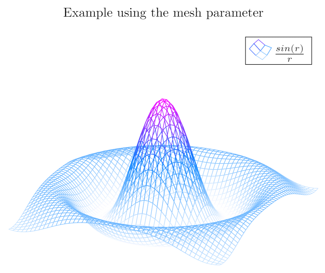
There are only two new things in this example: first, the samples y=0 to prevent pgfplots from joining the extreme points of the spiral and; second, the way the function to plot is passed to the addplot3 environment. Each parameter function is grouped inside curly brackets and the three parameters are delimited with a parenthesis.

The parameters passed to the axis and addplot environments can also be used in a data plot, except for scatter. Below the description of the code:

A také sadu nářadí, ke které budete potřebovat ještě hever a klíč na kola. Tlumiče se totiž nenastavují tlačítkem v autě nebo na displeji infotainmentu, ale pěkně postaru přímo na tělese tlumiče. Což znamená, že kola musí dolů (přesněji tedy u předních tlumičů stačí otevřít kapotu ke změně nastavení odskoku, k nastavení tlumení by mohlo stačit vytočit kolo, ale u zadních to bez sundání kol nepůjde). Většina majitelů se tak ani nebude snažit cokoliv měnit a všechny ty přednášky o změně charakteristiky tlumičů a jejich vlivu na chování auta si nechají do hospody pro oblbování kamarádů u piva.

To add an actual plot, the command \addplot[color=red]{log(x)}; is used. Inside the square brackets, [...], some options can be passed in; here, we set the color of the plot to red. The square brackets are mandatory, if no options are passed leave a blank space between them. Inside the curly brackets you put the function to plot. Is important to remember that this command must end with a semicolon (;).

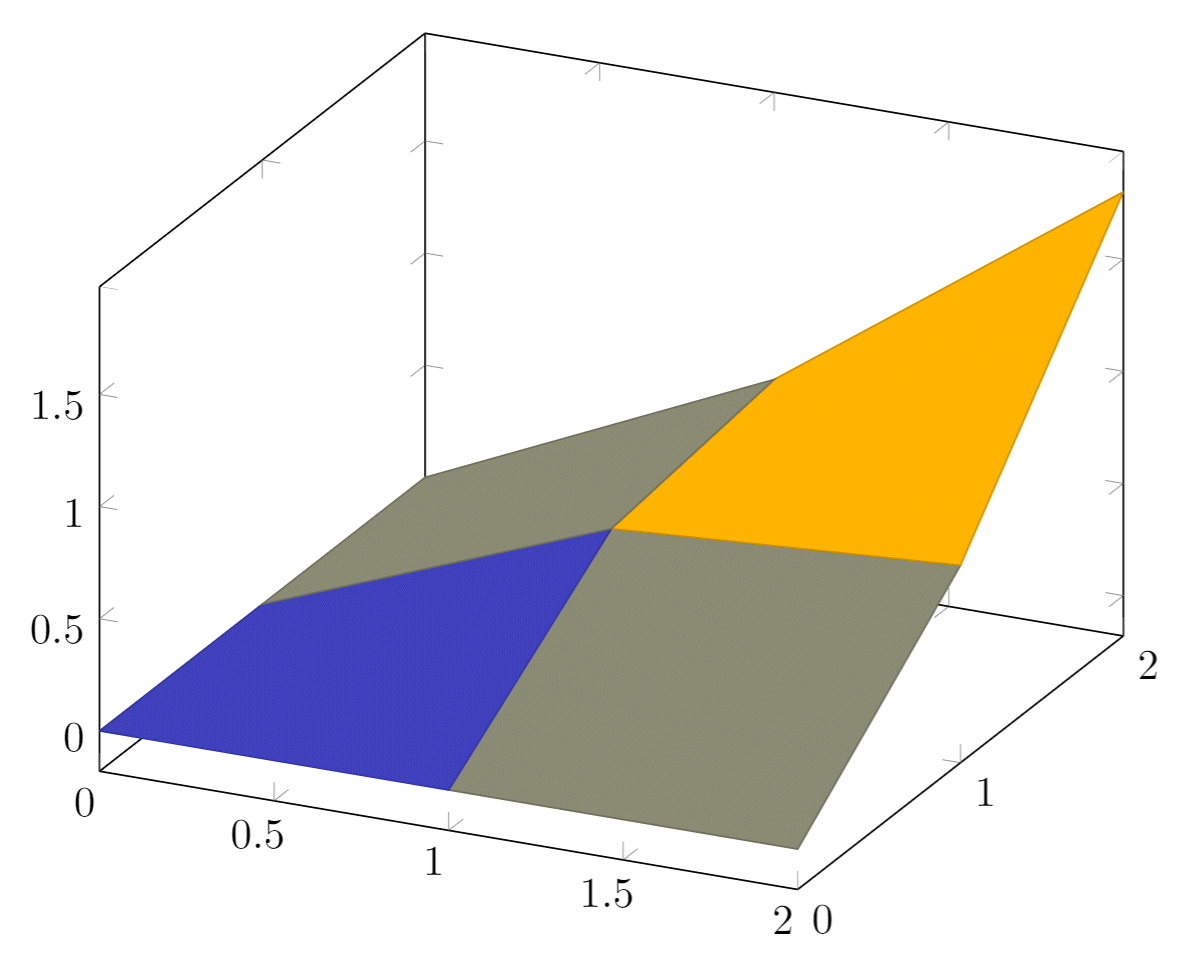
To plot a set of data into a 3D surface all we need is the coordinates of each point. These coordinates could be an unordered set or, in this case, a matrix:

You also can configure the behaviour of pgfplots in the document preamble. For example, to change the size of each plot and guarantee backwards compatibility (recommended) add the next line:

To increase speed of document-compilation you can configure the pgfplots package to export the figures to separate PDF files and then import them into the document: compile once, then re-use the figures. To do that, add the code shown below to the preamble:

The output from this code is shown in the image below—the LaTeX document preamble is added automatically when you open the link:

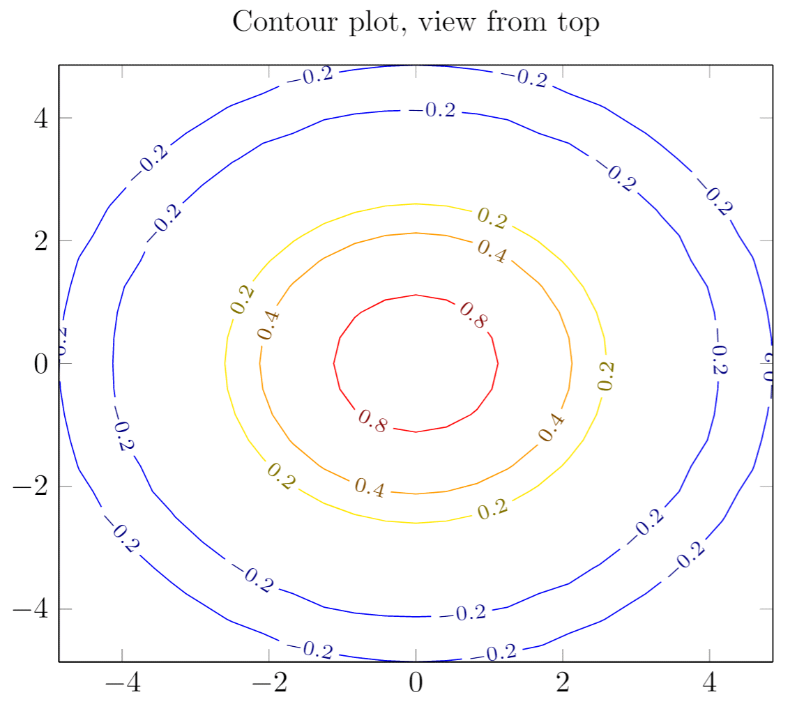
In pgfplots it is possible to plot contour plots, but the data has to be pre-calculated by an external program. Let's see an example:

Základní Competition za 234 tisíc vám přinese 20“ kola a hlučnější RS výfuk, posunutí limitu maximálky z 250 km/h na 290, Matrix LED světlomety a top LED koncová světla, k tomu paket černé optiky zvenku a uvnitř sedadla čalouněná mikrovláknem Dinamica a kůží.

Note: It's recommended as a good practice to indent the code—see the second plot in the example above—and to add a comma (,) at the end of each option passed to \addplot. This way the code is more readable and is easier to add further options if needed.

The pgfplots package, which is based on TikZ, is a powerful visualization tool and ideal for creating scientific/technical graphics. The basic idea is that you provide the input data/formula and pgfplots does the rest.

Vyšší Competition plus za 325 tisíc k tomu navíc přihodí dynamické řízení, sportovní diferenciál a právě zmíněné tlumiče. Volba je celkem jasná, co říkáte…?

Příplatkový podvozek i v základním nastavení funguje skvěle. A pokud vám jeho charakteristika nevyhovuje, můžete si ji přenastavit podle přání.

Už jen proto, že máte pod pravým chodidlem na povel 450 koní, které vás z klidu na stovku vystřelí za brutálních 3,8 sekundy za burácení a vytí dvakrát přeplňovaného šestiválce, který také rád střílí do výfuku a vůbec se vehementně snaží, abyste se za volantem nenudili. Přitom se ale umí také zklidnit a ztišit a jezdit dálky pod devět litrů.

The labels on the y-axis will show up to 4 digits. If the numbers you are working with are greater than 9999 pgfplots will use the same notation as in the example.

This changes the size of each pgfplot figure to 10 centimeters, which is huge; you may use different units (pt, mm, in). The compat parameter is for the code to work on the package version 1.9 or later.

Audi tak k modelům RS4 a RS5 dodává příplatkový Competition Pack s pasivními tlumiči, které však mají třícestné manuální nastavení jako u skutečného závoďáku – kromě snížení světlé výšky (o 10 mm, přitom už ve standardu je s těmito tlumiči o 10 mm nižší) si můžete upravit tlumení i odskok hned v několika krocích.

This is a plot of some contour lines for the same equation used in the previous section. The value of the title parameter is inside curly brackets because it contains a comma, so we use the grouping brackets to avoid any confusion with the other parameters passed to the \begin{axis} declaration. There are two new commands:

The output from this code is shown in the image below—the LaTeX document preamble is added automatically when you open the link:

The output from this code is shown in the image below—the LaTeX document preamble is added automatically when you open the link:

Because pgfplots is based on tikz the plot must be inside a tikzpicture environment. Then the environment declaration \begin{axis}, \end{axis} will set the correct scaling for the plot—check the Reference guide for other axis environments.

Scatter plots are used to represent information by using some kind of marks and are commonly used when computing statistical regression. In this example we'll create a scatter plot using data contained in a file called scattered_example.dat, in which the data looks like this:

The points passed to the coordinates parameter are treated as contained in a 3 × 3 matrix, using a blank line as the separator for each matrix row.

Víte přesně, jak funguje tlumič? Co je komprese a odskok a jaký vliv má na jízdní vlastnosti auta? Pokud ne, tak se tímhle článkem vůbec netrapte a objednejte si RS5 s adaptivním podvozkem, kde si tlačítkem v kabině přepnete mezi komfortním a sportovním nastavením podvozku – a budete nesmírně spokojení. Ale pokud se v autě rádi vrtáte a jako skvělí testovací piloti poznáte jemné nuance jemného nastavení, pak potřebujete něco lepšího…

The output from this code is shown in the image below—the LaTeX document preamble is added automatically when you open the link:

The output from this code is shown in the image below—the LaTeX document preamble is added automatically when you open the link:

pgfplots' 2D plotting functionalities are vast—and you can personalize your plots to suit your requirements. Nevertheless, the default options usually give very good results, so all you need to do is feed the data and LaTeX will do the rest.

Základní cena Audi RS5 Sportback činí 2 486 900 Kč, ale můžete ji vesele šroubovat nahoru přidáváním prvků příplatkové výbavy, ke kterým patří i balíčky Competition (233 900 Kč) a Competition Plus (324 700 Kč).

Nejostřejší RS5 Sportback tak dokáže trochu klamat tělem. Má čtyři dveře, čtyři plnohodnotná místa a 480litrový kufr k tomu, spoustu digitálních technologií a komfortní výbavy, automatickou převodovku a talent pro pohodové překonávání kontinentů, ale pozorného pozorovatele neoblbne – jen se podívejte na všechny ty průduchy a ostré linky, na ta lehká kola s nizoučkými šlupičkami, na ty macaté koncovky výfuku připomínající spíš hlavně houfnic. Na povel se celé auto našponuje a vystřelí vás po okresce tak rychle, až bude váš spolujezdec kvičet strachy!

A skvělé je, že si tohohle silničního rychlíka můžete nabrousit podle vlastních preferencí. Už v základu funguje skvěle, s paketem Competition je ještě atraktivnější a s technickými doplňky balíčku Competition Plus je pak prostě brilantní.

Ale ani to nevadí, protože tyhle tlumiče jsou už v základním nastavení skvělé! Přirozeně tužší, jak se na správné sportovní auto sluší a patří, přitom dost poddajné, aby z vás ani na českých okreskách nevytřásly duši. Spolu s lepivými pneumatikami Pirelli P Zero Corsa o rozměru 275/30 R20 tak máte spoustu přilnavosti, o kterou se můžete opřít, přitom pořád vnímáte drobné náklony auta jemně zdůrazňující, co se právě děje.

If the data is in a file, which is the case most of the time; instead of the commands \addplot and coordinates you should use \addplot table {file_with_the_data.dat}, the rest of the options are valid in this environment.

Obsah serveru je chráněn autorským právem. Jakékoli užití obsahu serveru včetně publikování nebo jiného šíření obsahu serveru je bez písemného souhlasu těchto společností zakázáno.

When the original TeX engine was conceived/written, more than 40 years ago, it was not designed for direct production of graphics—those were to be files created by external programs (e.g., MetaPost) and imported into the typeset document. The advent of pdfTeX—which is closely based on the original TeX software—brought the ability to create graphics directly by using pdfTeX's new built-in TeX language commands (called primitives) which can output the PDF operators/data required to produce graphics. The creation of pdfTeX led to the development of sophisticated LaTeX graphics packages, such as TikZ, pgfplots etc, capable of producing graphics coded using high-level LaTeX commands.

The figure starts with the (previously explained) declaration of the tikzpicture and axis environments, but the axis declaration has a number of new parameters: